Mobility

This module deals with the process of measuring human mobility through Twitter’s data. It processes the information provided by Twitter and provides the displacement in different ways, such as the number of travels in an origin-destination matrix, the overall mobility, and the outward mobility.

To illustrate the library’s use, let us produce mobility plots on the period contemplating from February 15, 2020, to July 12, 2020. The following code retrieved the mobility information on the specified period.

>>> from text_models import Mobility
>>> start = dict(year=2020, month=7, day=12)
>>> end = dict(year=2020, month=2, day=15)
>>> mob = Mobility(start, end=end)

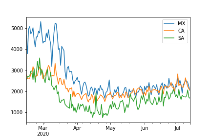
Let us start presenting mobility as the number of travels in Mexico, Canada, and Saudi Arabia. The following code computes the mobility in all the countries. The first line counts the trips that occurred within the country as well as the inward and outward movement. The information is arranged in a DataFrame or a dictionary, depending on whether the pandas’ flag is activated. The second line generates the plot for the countries of interest, i.e., Mexico (MX), Canada (CA), Saudi Arabia (SA).

>>> data = mob.overall(pandas=True)
>>> data[["MX", "CA", "SA"]].plot()

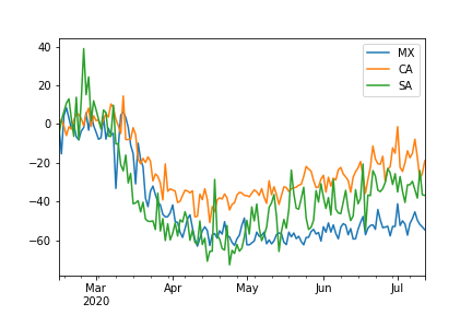
An approach to transforming the mobility information from a number of trips into a percentage is by using a baseline period. The baseline statistics can be computed using different procedures; one uses the weekday, and the other uses a clustering algorithm, particularly k-means. The text_models library has two classes; one computes the percentage using weekday information, namely text_models.place.MobilityWeekday, and the other using a clustering algorithm, i.e., text_models.place.MobilityCluster. The following code computes the percentage using the weekday information; the code is similar to the one used to produce the previous figure being the only difference the class used.

>>> from text_models import MobilityWeekday
>>> mob = MobilityWeekday(start, end=end)
>>> data = mob.overall(pandas=True)
>>> data[["MX", "CA", "SA"]].plot()

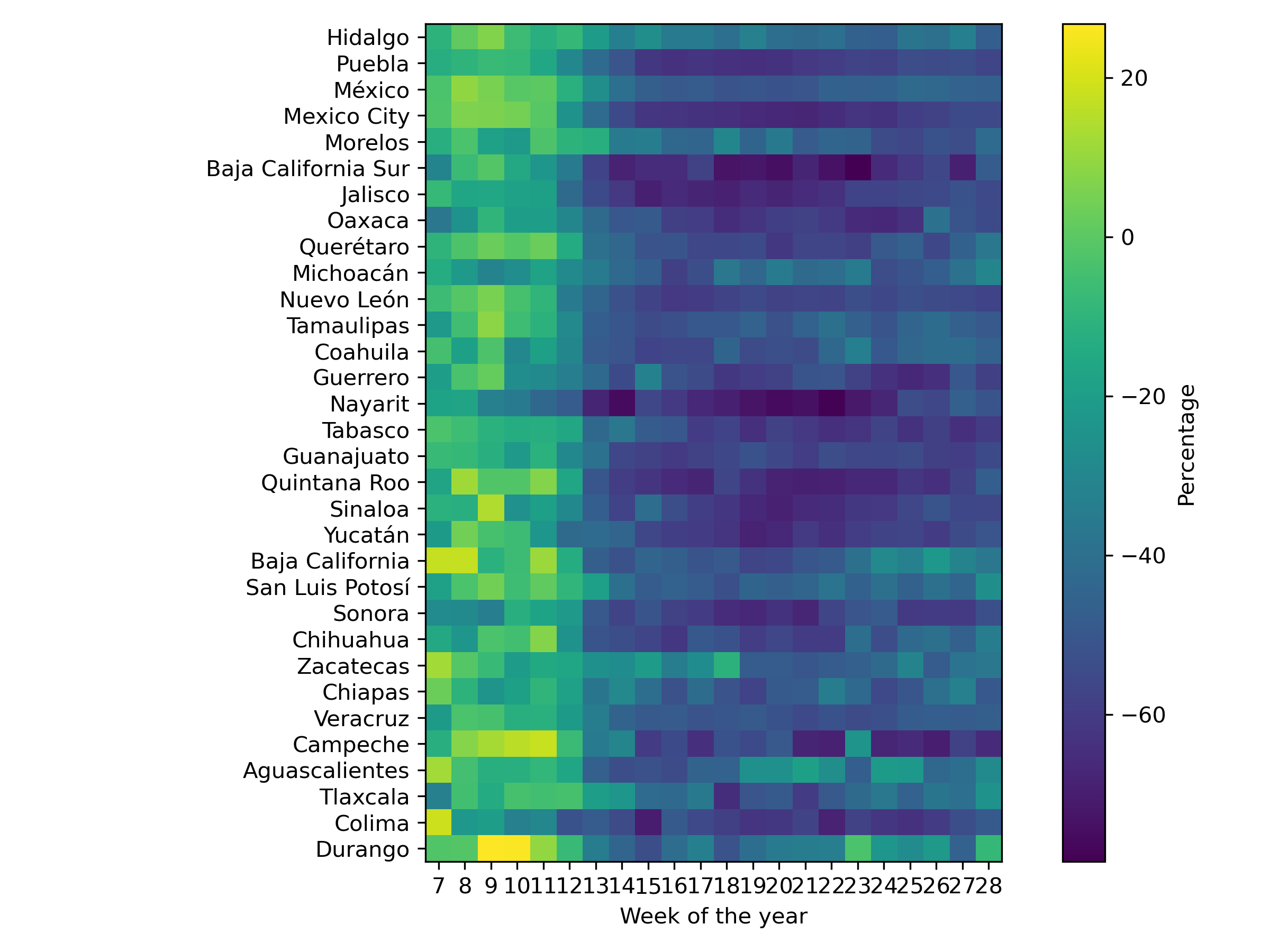
So far, we have seen a procedure to compute the mobility using the number of travels and the percentage in different countries. In order to complement the approach, let us compute the mobility between Mexico’s states. The code is similar to the one used in the previous examples, being the difference that one needs to provide a function (argument level) that transforms the landmark identifier into a state identifier and filters the landmarks that do not correspond to Mexico.

>>> data = mob.overall(level=lambda x: mob.state(x) if x[:3] == "MX:" else None, pandas=True)

Let us create a heat map to represent the mobility of all states into one figure. The first step is to resample the information to present average mobility in a week. Then, the mobility information is transposed to represent the states as rows and the weeks as columns.

>>> dd = data.resample("W").mean()
>>> unico = dd.T
>>> index = unico.index.to_numpy()
>>> columns = unico.columns
>>> unico = unico.to_numpy()

In order to write the state name instead of the identifier, we use the following class.

>>> from text_models.place import States
>>> states = States()

It is time to create the heatmap; the following code creates the heatmap.

>>> from matplotlib import pylab as plt
>>> fig = plt.figure(figsize=(8, 6), dpi=300)
>>> ax = fig.subplots()
>>> _ = ax.imshow(unico, cmap="viridis")
>>> cbar = fig.colorbar(_, ax=ax, orientation="vertical", shrink=1)
>>> cbar.set_label('Percentage', rotation=90)
>>> _ = plt.yticks(range(index.shape[0]), [states.name(x) for x in index])
>>> _ = plt.xticks(range(len(columns)), [x.weekofyear for x in columns])
>>> plt.xlabel("Week of the year")
>>> plt.tight_layout()
>>> plt.savefig("heatmap.png")

To complement the overview of the information that can be obtained from this module, we refer the reader to the notebook.

Using your Tweets

The previous steps assumed the use of the mobility data collected and transform by ingeotec. However, sometimes one would like to use the algorithms developed in data collected with different characteristics. Let us assume the tweets are in a file called “tweets.json.gz”; the format is one JSON per line. In the tests, it is available some collected tweets to make this example self-contained. These tweets are on the following path.

>>> from text_models.tests import test_place
>>> from os.path import join
>>> DIR = test_place.DIR
>>> fname = join(DIR, "tweets.json.gz")

Then to create the origin-destination matrix used by text_models.place.Mobility, the following code can be used.

>>> from text_models.place import OriginDestination
>>> ori_dest = OriginDestination(fname)
>>> ori_dest.compute("210604.travel")

It is also possible to use a list of files instead of just one, so it is acceptable that the parameter fname would be a list. Furthermore, it might be the case that the file has a different format, so it is also possible to give a function (reader) that returns an iterable object where each element is a dictionary with the same format used by Twitter.

The last part is to use the origin-destination matrix (i.e., “210604.travel”) in the text_models.place.Mobility. To do so, it is needed to replace the method used to find the mobility information, this is provided by the parameter data. The following code illustrates this process.

>>> from text_models.place import Mobility
>>> data = lambda x: join(".", x)
>>> mob = Mobility(day=dict(year=2021, month=6, day=4), window=1, data=data)
>>> dd = mob.overall(pandas=True)

text_models.place

class text_models.place.BoundingBox

The lowest resolution, on mobility, is the centroid of the bounding box provided by Twitter. Each centroid is associated with a label. This class provides the mapping between the geo-localization and the centroid’s label.

property bounding_box

Bounding box data

city(label)

Mexico cities

property coords

Bounding box’s coordinates

label(data)

The label of the closest bounding-box centroid to the data

Parameters

data (dict) – A dictionary containing the country and the position

>>> from text_models.place import BoundingBox
>>> bbox = BoundingBox()
>>> bbox.label(dict(country="MX", position=[0.34387610272769614, -1.76610232121455]))
'MX:6435'

property pc

Postal code

postal_code(label)

Mexico postal code given a label

Parameters

label (str) – Bounding box label

>>> from text_models.place import BoundingBox
>>> bbox = BoundingBox()
>>> bbox.postal_code('MX:6435')
'58000'

class text_models.place.CP

Mexico Postal Codes

>>> from text_models.place import CP
>>> cp = CP()
>>> tw = dict(coordinates=dict(coordinates=[-99.191996,19.357102]))
>>> cp.convert(tw)
'01040'
>>> box = dict(place=dict(bounding_box=dict(coordinates=[[[-99.191996,19.357102],[-99.191996,19.404124],[-99.130965,19.404124],[-99.130965,19.357102]]])))
>>> cp.convert(box)
'03100'

convert(x: dict) → str

Obtain the postal code from a tweet

Parameters

x (dict) – Tweet

Returns

Postal Code

Return type

str

postal_code(lat: float, lon: float, degrees=True) → str

Postal code

Parameters

• lat (float) – Latitude

• lon (float) – Longitude

• degrees (bool) – Indicates whether the point is in degrees

>>> from text_models.place import CP
>>> cp = CP()
>>> cp.postal_code(19.357102, -99.191996)
'01040'

property postal_code_names

Dictionary containing a descripcion of a postal code

>>> from text_models.place import CP
>>> cp = CP()
>>> cp.postal_code_names["58000"]
['16', 'Michoacán de Ocampo', '053', 'Morelia']

state(postal_code)

>>> from text_models.place import CP
>>> cp = CP()
>>> cp.state("20900")
'Aguascalientes'

class text_models.place.Country

Obtain the country from a text.

>>> from text_models.place import Country
>>> cntr = Country()
>>> cntr.country("I live in Mexico.")
'MX'

country(text)

Identify a country in a text

Parameters

text (str) – Text

Returns

The two letter country code

country_from_twitter(tw)

Identify the country from a tweet.

Parameters

tw (dict) – Tweet

class text_models.place.Mobility(day=None, window=30, end=None, data: ~typing.Callable[[str], str] = <function download_geo>, countries: ~typing.Optional[set] = None)

Mobility on twitter

Parameters

• day (datetime) – Starting day default yesterday

• window (int) – Window used to perform the analysis

• end (datetime) – End of the period, use to override window.

• data – Path to the origin destination matrix

• countries (set) – Set of countries on analysis (None: all)

>>> from text_models.place import Mobility
>>> mobility = Mobility(window=5)
>>> output = mobility.overall(level=mobility.state)

property bounding_box

Bounding box

cluster_percentage(data, n_clusters=None)

Compute the percentage using KMeans with K=7.

Parameters

• data (dict) – Data, e.g., text_models.place.Mobility.inside_mobility()

• n_clusters (int or function) – Number of function to maximize

Return type

dict

country(key)

Country that correspond to the key.

>>> from text_models.place import Mobility
>>> mobility = Mobility(window=1)
>>> mobility.country('MX:6435')
'MX'

create_transform(data, transformation)

Instantiate the transform class

property dates

Dates used on the analysis

displacement(level=None)

Displacement matrix

Parameters

level – Aggregation function

static fill_with_zero(output)

Fill mobility matrix with zero when a particular destination is not present.

group_by_weekday(data)

Group the data by weekday works on a list of dictionaries where the value of the dictionary is a number.

Parameters

data (list) – List of dictionaries, e.g., text_models.place.Mobility.inside_mobility()

Return type

dict

inside_mobility(level=None, pandas=False)

Mobility inside the region defined by level

Parameters

• level – Aggregation function

• pandas (bool) – Mobility as a DataFrame

inside_outward(level)

Inside and outward mobility

Parameters

level – Aggregation function

static keep_only(data, countries: Optional[set] = None)

Keep only the countries, do nothing when len(countries) is zero.

outward(level=None)

Outward mobility in an origin-destination matrix

Parameters

level – Aggregation function

Return type

list

overall(level=None, pandas=False)

Overall mobility, this counts for outward, inward and inside travels in the region of interest (i.e., level).

Parameters

• level (function) – Aggregation function

• pandas (bool) – Mobility as a DataFrame

state(label, mex=False)

State that correspons to the label.

Parameters

• label (str) – Label of the point

• mex_pc (bool) – Use Mexico’s state identifier

>>> from text_models.place import Mobility
>>> mobility = Mobility(window=1)
>>> mobility.state('MX:6435', mex=True)
'16'
>>> mobility.state("CA:12")
'CA-ON'
>>> mobility.state("MX:0")
'MX-CHP'

transform(data, baseline)

Transform data using the baseline

Parameters

• data (dict) – Mobility data

• baseline (dict) – Baseline used to compute the percentage, e.g., text_models.place.Mobility.median_weekday()

property travel_matrices

List of origin-destination matrix

weekday_percentage(data)

Compute the percentage of each weekday using the median.

Parameters

data (dict) – Data, e.g., text_models.place.Mobility.displacement()

Return type

dict

weekday_probability(data)

Normal distribution of weekday data.

Parameters

data (dict) – Data, e.g., text_models.place.Mobility.inside_mobility()

Return type

dict

class text_models.place.MobilityCluster(day=None, baseline=91, n_clusters=<function silhouette_score>, **kwargs)

Represent mobility as the percentage of change using KMeans to create the baseline information.

Parameters

• baseline (int) – Number of days to create the baseline

• n_clusters (int | func) – Either the number of clusters is given or a function to maximize

property baseline

Baseline used to compute the percentage

inside_mobility(level=None, pandas=False)

Mobility inside the region defined by level

Parameters

• level – Aggregation function

• pandas (bool) – Mobility as a DataFrame

overall(level=None, pandas=False)

Overall mobility, this counts for outward, inward and inside travels in the region of interest (i.e., level).

Parameters

• level (function) – Aggregation function

• pandas (bool) – Mobility as a DataFrame

class text_models.place.MobilityWeekday(day=None, baseline=91, **kwargs)

Represent mobility as the percentage of change using the weekday information as the baseline

Parameters

baseline (int) – Number of days to create the baseline

property baseline

Baseline used to compute the percentage

inside_mobility(level=None, pandas=False)

Mobility inside the region defined by level

Parameters

• level – Aggregation function

• pandas (bool) – Mobility as a DataFrame

overall(level=None, pandas=False)

Overall mobility, this counts for outward, inward and inside travels in the region of interest (i.e., level).

Parameters

• level (function) – Aggregation function

• pandas (bool) – Mobility as a DataFrame

class text_models.place.OriginDestination(fnames: ~typing.Union[list, str], reader: ~typing.Callable[[str], ~typing.Iterable[dict]] = <function tweet_iterator>)

Compute the origin-destination matrix. It starts from a list of files where each line is a JSON, using the same structure as Twitter. The following code is a working example. :param fnames: List or str :param reader: Function to read each file

>>> from text_models.place import OriginDestination
>>> from text_models.tests import test_place
>>> from os.path import join
>>> DIR = test_place.DIR
>>> fname = join(DIR, "tweets.json.gz")
>>> ori_dest = OriginDestination(fname)
>>> ori_dest.compute("210604.travel")

class text_models.place.States

Auxiliary function to retrieve the States or Provinces geometries and attributes from Natural Earth.

associate(data, country=None)

Associate a array of points with the states.

Parameters

• data (list) – Array of points in radians (lat, lon)

• country (str) – Country using two letters code

text_models.place.Travel

alias of Mobility

text_models.place.distance(lat1: float, lng1: float, lat2: float, lng2: float) → float

Taken from http://www.samuelbosch.com/2018/09/great-circle-calculations-with-numpy.html also available at: https://raw.githubusercontent.com/samuelbosch/blogbits/master/geosrc/numpy_greatcircle.py

text_models.place.length(x: dict) → float

Bounding box length

Parameters

x (dict) – Tweet

Return type

float

>>> from text_models.place import length
>>> bbox = dict(place=dict(bounding_box=dict(coordinates=[[[-99.191996,19.357102],[-99.191996,19.404124],[-99.130965,19.404124],[-99.130965,19.357102]]])))
>>> l = length(bbox)
>>> "{:0.4f}".format(l)
'8.2657'

text_models.place.location(x: dict) → Tuple[float, float]

Location of a tweet. In the case, it is a bounding box the location is the average.

Parameters

x (dict) – Tweet

Return type

tuple

text_models.place.point(longitude: float, latitude: float) → Tuple[float, float]

Transform longitude and latitude from degrees to radians, and reverse the order, i.e., latitude and longitude.